Introduction to Non-linear Data Structures

Non-linear Data Structures

Non-linear data structures are those that are not organized in a line or sequential order. Instead, the data elements are structured in a network-based format. Non-linear data structures tend to be more intricate to set up than linear data structures. They can offer efficiency for specific tasks, like searching and sorting. It is a non-primitive type.

In this Data structures tutorial, we will go through non-linearData Structures including Trees,Graphs,Hash Tables,Sets, andProperties of Non-Linear Data Structures.

Explain Non-Linear Data Structure

• In data structures, a non-linear data structure stands out as a type where elements are not placed in a sequence.
• Unlike structures, like arrays stacks, and queues.
• The arrays stacks and queues that adhere to an order of non-linear data structures arrange information, in hierarchical or graphical formats.
• They enable intricate connections and streamlined data organization.

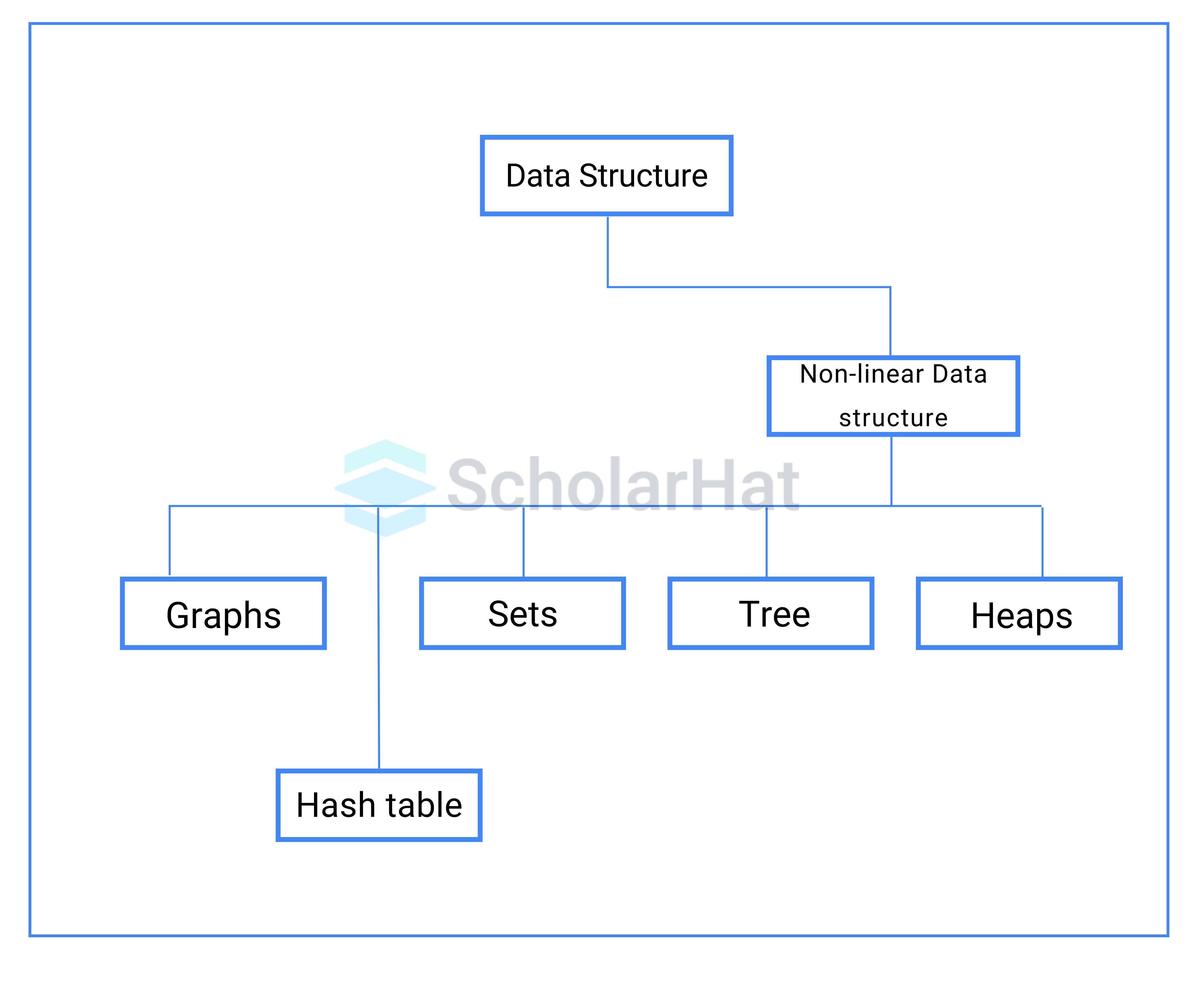
There are various Non-Linear Data Structures. They are as follows:

• Tree
• Graph

Trees

• The tree is formed entirely of various nodes and is a non-linear data structure.
• The tree data structure's nodes are grouped hierarchically.
• It is made up of a root node that corresponds to all of its different child nodes that are at the next level.
• The tree grows levelly, with root nodes having a finite number of child nodes based on the tree's order.
• Since a tree data structure doesn't store information sequentially, because, it is non-linear.
• The arrangement of items in a tree is hierarchical, with levels within the tree.
• A root node is the highest node in a tree data structure.
• Every node has some data, which can be any kind of data.

Types of Trees

There are various types of trees in non-linear data structures, They are as follows:

• Binary Tree
• Simple Tree
• Complete Binary tree
• Binary Search Tree
• AVL Trees
• B -Tree
• B+ Tree

Let's discuss some types of trees below

1. Simple tree

• A simple tree is only an N-array tree with a root node and several offspring nodes.
• The tree grows in this manner because the child nodes are present on the root node at the next level.
• We can create a basic tree with no limitations on the offspring of the root node.
• A generic tree is any tree that has a hierarchical structure.
• The absence of any configuration or restrictions on the maximum number of children a node may have defines a general tree.
• Any combination of these can be the orientation of the tree, and a node can have any number of children.
• The nodes' degrees might vary from 0 to n.

2. Binary tree

• This subclass of simple trees is crucial.
• As the name implies, it should come as no surprise that the binary tree only has two children.
• By definition, a binary tree consists of nodes that are capable of bearing two children, as indicated by the term "binary," which stands for "two numbers."
• In a binary tree, a node may contain a maximum of 0, 1, or 2 nodes.
• Binary trees in data structures are highly useful ADTs that fall into many categories.
• Binary trees are those whose constituents have no more than two children.
• We usually refer to the left and right children as such since each element in a binary tree can only have two children.
• Most frequently, they are employed in data structures for

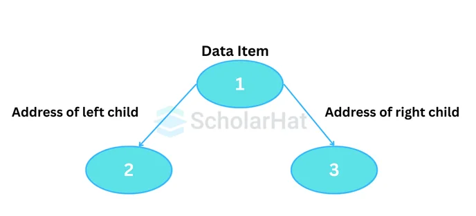
A Binary tree is represented by a pointer to the topmost node known as the root node. If the tree is empty, the value of the root is NULL. Each node of a Binary Tree contains the following three elements:

• Data
• Pointer to the left child
• Pointer to the right child

Binary Tree Terminologies in Data Structures:

• Node: In a binary tree, a node refers to a data element stored in the tree. They contain the address of the left and right child.
• Root: In a binary tree, the root is the topmost node of the tree. It is the starting point of the tree from which all other nodes branch out. A tree can have at most one root node.
• Parent Node: A node (except the root) that has a succeeding node is known as a parent node.
• Child Node: A node that has a preceding node is known as a child node. A node can be both parent and child depending on the node that is in context.
• Leaf Node: A leaf node in a binary tree is a node that does not have any children i.e. terminal node in the tree.
• Internal Node: In a binary tree, an internal node is a node that has at least one child.
• Depth of a Tree: The depth of a tree in a binary tree refers to the length of the longest path from the root node to any leaf node in the tree.
• Height of a Tree: The number of edges from the deepest node in the tree to the root node.

Syntax

How to declare/create a Binary Tree in Data Structures? Let's see below,

struct node
{
 int data;
 struct node *left;
 struct node *right;
};

Implementation of a Binary Tree in Different Programming Languages

class Node:
    def __init__(self, key):
        self.left = None
        self.right = None
        self.val = key

    # Traverse preorder
    def traversePreOrder(self):
        print(self.val, end=' ')
        if self.left:
            self.left.traversePreOrder()
        if self.right:
            self.right.traversePreOrder()

    # Traverse inorder
    def traverseInOrder(self):
        if self.left:
            self.left.traverseInOrder()
        print(self.val, end=' ')
        if self.right:
            self.right.traverseInOrder()

    # Traverse postorder
    def traversePostOrder(self):
        if self.left:
            self.left.traversePostOrder()
        if self.right:
            self.right.traversePostOrder()
        print(self.val, end=' ')


root = Node(5)

root.left = Node(6)
root.right = Node(7)

root.left.left = Node(8)

print("Preorder Traversal: ", end="")
root.traversePreOrder()
print("\nInorder Traversal: ", end="")
root.traverseInOrder()
print("\nPostorder Traversal: ", end="")
root.traversePostOrder()
    

// Node creation
class Node {
  int key;
  Node left, right;

  public Node(int item) {
  key = item;
  left = right = null;
  }
}

class BinaryTree {
  Node root;

  BinaryTree(int key) {
  root = new Node(key);
  }

  BinaryTree() {
  root = null;
  }

  // Traverse Inorder
  public void traverseInOrder(Node node) {
  if (node != null) {
    traverseInOrder(node.left);
    System.out.print(" " + node.key);
    traverseInOrder(node.right);
  }
  }

  // Traverse Postorder
  public void traversePostOrder(Node node) {
  if (node != null) {
    traversePostOrder(node.left);
    traversePostOrder(node.right);
    System.out.print(" " + node.key);
  }
  }

  // Traverse Preorder
  public void traversePreOrder(Node node) {
  if (node != null) {
    System.out.print(" " + node.key);
    traversePreOrder(node.left);
    traversePreOrder(node.right);
  }
  }

  public static void main(String[] args) {
  BinaryTree tree = new BinaryTree();

  tree.root = new Node(5);
  tree.root.left = new Node(6);
  tree.root.right = new Node(7);
  tree.root.left.left = new Node(8);

  System.out.print("Preorder Traversal: ");
  tree.traversePreOrder(tree.root);
  System.out.print("\nInorder Traversal: ");
  tree.traverseInOrder(tree.root);
  System.out.print("\nPostorder Traversal: ");
  tree.traversePostOrder(tree.root);
  }
}
    

#include <stdlib.h>
#include <iostream>
using namespace std;

struct node {
  int data;
  struct node *left;
  struct node *right;
};

// New node creation
struct node *newNode(int data) {
  struct node *node = (struct node *)malloc(sizeof(struct node));

  node->data = data;

  node->left = NULL;
  node->right = NULL;
  return (node);
}

// Traverse Preorder
void traversePreOrder(struct node *temp) {
  if (temp != NULL) {
    cout << " " << temp->data;
    traversePreOrder(temp->left);
    traversePreOrder(temp->right);
  }
}

// Traverse Inorder
void traverseInOrder(struct node *temp) {
  if (temp != NULL) {
    traverseInOrder(temp->left);
    cout << " " << temp->data;
    traverseInOrder(temp->right);
  }
}

// Traverse Postorder
void traversePostOrder(struct node *temp) {
  if (temp != NULL) {
    traversePostOrder(temp->left);
    traversePostOrder(temp->right);
    cout << " " << temp->data;
  }
}

int main() {
  struct node *root = newNode(5);
  root->left = newNode(6);
  root->right = newNode(7);
  root->left->left = newNode(8);

  cout << "preorder traversal: ";
  traversePreOrder(root);
  cout << "\nInorder traversal: ";
  traverseInOrder(root);
  cout << "\nPostorder traversal: ";
  traversePostOrder(root);
}
    

Output

Preorder traversal:  5 6 8 7
Inorder traversal:  8 6 5 7
Postorder traversal:  8 6 7 5

3. Binary Search Tree

• A subtype of a binary tree is known as a Binary Search Tree (BST).
• It is set up so that the parent node's left subnode is always smaller than the parent node and the parent node's right subnode is always larger than the parent node.
• It is the altered form of the binary tree, and it grows in a similar manner.
• Binary search trees are more restricted than binary trees.
• Unlike binary trees, which require us to retain the 0, 1, or 2 children of each node.
• It also needs us to maintain a specific order for the insertion of child nodes.

Special Characteristics of Binary Search Tree

These properties differentiate a Binary Search tree from a Binary tree.

1. The keys of nodes in the left subtree of a node are less than the node’s key.
2. The keys of nodes in the right subtree of a node are greater than the node’s key.
3. Both subtrees of each node are also BSTs i.e. they have the above two features.

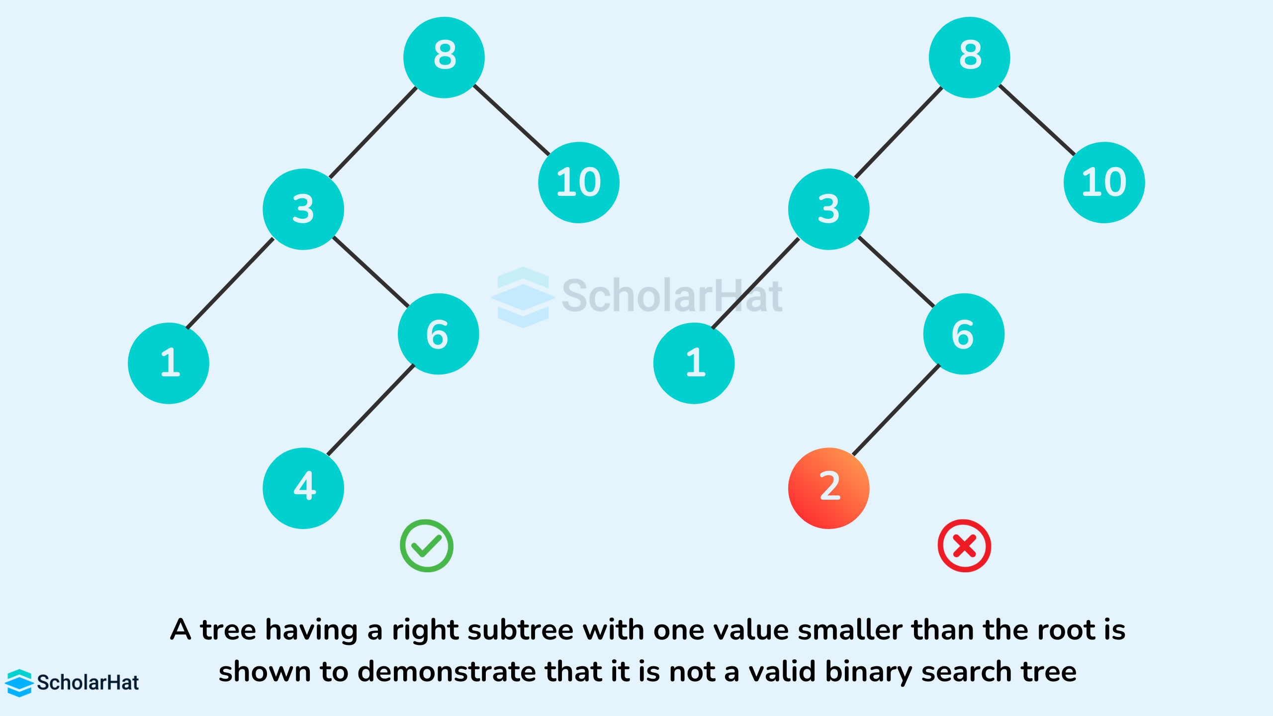
The binary tree on the right isn't a binary search tree because the right subtree of the node "3" contains a value smaller than it.

Read More: Data Structure Interview Questions and Answers

Implementation of Binary Search Trees in Different Programming Languages

class Node:
    def __init__(self, key):
        self.key = key
        self.left = None
        self.right = None

# Inorder traversal
def inorder(root):
    if root is not None:
        # Traverse left
        inorder(root.left)

        # Traverse root
        print(str(root.key) + "->", end=' ')

        # Traverse right
        inorder(root.right)


# Insert a node
def insert(node, key):

    # Return a new node if the tree is empty
    if node is None:
        return Node(key)

    # Traverse to the right place and insert the node
    if key < node.key:
        node.left = insert(node.left, key)
    else:
        node.right = insert(node.right, key)

    return node


# Find the inorder successor
def minValueNode(node):
    current = node

    # Find the leftmost leaf
    while(current.left is not None):
        current = current.left

    return current


# Deleting a node
def deleteNode(root, key):

    # Return if the tree is empty
    if root is None:
        return root

    # Find the node to be deleted
    if key < root.key:
        root.left = deleteNode(root.left, key)
    elif(key > root.key):
        root.right = deleteNode(root.right, key)
    else:
        # If the node is with only one child or no child
        if root.left is None:
            temp = root.right
            root = None
            return temp

        elif root.right is None:
            temp = root.left
            root = None
            return temp

        # If the node has two children,
        # place the inorder successor in position of the node to be deleted
        temp = minValueNode(root.right)

        root.key = temp.key

        # Delete the inorder successor
        root.right = deleteNode(root.right, temp.key)

    return root


root = None
root = insert(root, 9)
root = insert(root, 3)
root = insert(root, 2)
root = insert(root, 4)
root = insert(root, 7)
root = insert(root, 10)
root = insert(root, 15)
root = insert(root, 5)

print("Inorder traversal: ", end=' ')
inorder(root)

print("\nDelete 10")
root = deleteNode(root, 10)

print("Inorder traversal: ", end=' ')
inorder(root)
    

class Node {
    int key;
    Node left, right;

    public Node(int item) {
        key = item;
        left = right = null;
    }
}

public class BinaryTree {
    Node root;

    BinaryTree() {
        root = null;
    }

    // Inorder traversal
    void inorder(Node root) {
        if (root != null) {
            // Traverse left
            inorder(root.left);

            // Traverse root
            System.out.print(root.key + "-> ");

            // Traverse right
            inorder(root.right);
        }
    }

    // Insert a node
    Node insert(Node root, int key) {
        // Return a new node if the tree is empty
        if (root == null) {
            return new Node(key);
        }

        // Traverse to the right place and insert the node
        if (key < root.key) {
            root.left = insert(root.left, key);
        } else {
            root.right = insert(root.right, key);
        }

        return root;
    }

    // Find the inorder successor
    Node minValueNode(Node root) {
        Node current = root;

        // Find the leftmost leaf
        while (current.left != null) {
            current = current.left;
        }

        return current;
    }

    // Deleting a node
    Node deleteNode(Node root, int key) {
        // Return if the tree is empty
        if (root == null) {
            return root;
        }

        // Find the node to be deleted
        if (key < root.key) {
            root.left = deleteNode(root.left, key);
        } else if (key > root.key) {
            root.right = deleteNode(root.right, key);
        } else {
            // If the node is with only one child or no child
            if (root.left == null) {
                return root.right;
            } else if (root.right == null) {
                return root.left;
            }

            // If the node has two children,
            // place the inorder successor in position of the node to be deleted
            root.key = minValueNode(root.right).key;

            // Delete the inorder successor
            root.right = deleteNode(root.right, root.key);
        }

        return root;
    }

    public static void main(String[] args) {
        BinaryTree tree = new BinaryTree();
        tree.root = tree.insert(tree.root, 9);
        tree.root = tree.insert(tree.root, 3);
        tree.root = tree.insert(tree.root, 2);
        tree.root = tree.insert(tree.root, 4);
        tree.root = tree.insert(tree.root, 7);
        tree.root = tree.insert(tree.root, 10);
        tree.root = tree.insert(tree.root, 15);
        tree.root = tree.insert(tree.root, 5);

        System.out.print("Inorder traversal: ");
        tree.inorder(tree.root);
        System.out.println();

        System.out.println("Delete 10");
        tree.root = tree.deleteNode(tree.root, 10);

        System.out.print("Inorder traversal: ");
        tree.inorder(tree.root);
    }
}
    

#include <iostream>

// Create a node
class Node {
public:
    int key;
    Node* left;
    Node* right;

    Node(int k) : key(k), left(nullptr), right(nullptr) {}
};

// Inorder traversal
void inorder(Node* root) {
    if (root != nullptr) {
        // Traverse left
        inorder(root->left);

        // Traverse root
        std::cout << root->key << "-> ";

        // Traverse right
        inorder(root->right);
    }
}

// Insert a node
Node* insert(Node* node, int key) {
    // Return a new node if the tree is empty
    if (node == nullptr)
        return new Node(key);

    // Traverse to the right place and insert the node
    if (key < node->key)
        node->left = insert(node->left, key);
    else
        node->right = insert(node->right, key);

    return node;
}

// Find the inorder successor
Node* minValueNode(Node* node) {
    Node* current = node;

    // Find the leftmost leaf
    while (current->left != nullptr)
        current = current->left;

    return current;
}

// Deleting a node
Node* deleteNode(Node* root, int key) {
    // Return if the tree is empty
    if (root == nullptr)
        return root;

    // Find the node to be deleted
    if (key < root->key)
        root->left = deleteNode(root->left, key);
    else if (key > root->key)
        root->right = deleteNode(root->right, key);
    else {
        // If the node is with only one child or no child
        if (root->left == nullptr) {
            Node* temp = root->right;
            delete root;
            return temp;
        } else if (root->right == nullptr) {
            Node* temp = root->left;
            delete root;
            return temp;
        }

        // If the node has two children,
        // place the inorder successor in position of the node to be deleted
        Node* temp = minValueNode(root->right);

        root->key = temp->key;

        // Delete the inorder successor
        root->right = deleteNode(root->right, temp->key);
    }

    return root;
}

int main() {
    Node* root = nullptr;
    root = insert(root, 9);
    root = insert(root, 3);
    root = insert(root, 2);
    root = insert(root, 4);
    root = insert(root, 7);
    root = insert(root, 10);
    root = insert(root, 15);
    root = insert(root, 5);

    std::cout << "Inorder traversal: ";
    inorder(root);
    std::cout << std::endl;

    std::cout << "Delete 10" << std::endl;
    root = deleteNode(root, 10);

    std::cout << "Inorder traversal: ";
    inorder(root);
    std::cout << std::endl;

    return 0;
}
    

Output

Inorder traversal:  2-> 3-> 4-> 5-> 7-> 9-> 10-> 15-> 
Delete 10
Inorder traversal:  2-> 3-> 4-> 5-> 7-> 9-> 15-> 

Graphs

• A graph is a collection of nodes that consist of data and are connected to other nodes of the graph.
• formally a Graph is composed of a set of vertices( V ) and a set of edges( E ). The graph is denoted by G(V, E).
• The most common real-life examples of graphs are social media where a User, Photo, Album, Event, Group, Page, Comment, Story, Video, etc represents a node.
• Every relationship is an edge from one node to another.
• Whenever you post a photo, join a group, like a page, etc., a new edge is created for that relationship.
• Thus, it can be said that a social media platform is a collection of nodes and edges.

Graph Terminologies in Data Structures

Graph terminology in data structure refers to the specific vocabulary and concepts used to describe and analyze graphs, which are mathematical structures composed of nodes (also called vertices) connected by edges.

• Node/Vertex: A fundamental unit of a graph. It represents an entity or an element and is usually depicted as a point.
• Edge/Arc: A connection between two nodes. It represents a relationship or a link between the corresponding entities. An edge can be directed (arc), indicating a one-way connection, or undirected, representing a two-way connection.
• Adjacent Nodes: Two nodes that are directly connected by an edge. In an undirected graph, both nodes are considered adjacent to each other. In a directed graph, adjacency depends on the direction of the edge.
• Degree: The degree of a node is the number of edges incident to it, i.e., the number of edges connected to that node. In a directed graph, the degree is divided into two categories: the in-degree (number of incoming edges) and the out-degree (number of outgoing edges).
• Path: A path in a graph is a sequence of edges that connects a sequence of nodes. It can be a simple path (no repeated nodes) or a closed path/cycle (starts and ends at the same node).
• Bipartite Graph: A graph whose nodes can be divided into two disjoint sets such that every edge connects a node from one set to a node from the other set. In other words, there are no edges between nodes within the same set.
• Spanning Tree: A subgraph of a connected graph that includes all the nodes of the original graph and forms a tree (a connected acyclic graph) by eliminating some of the edges.
• Cycle: A closed path in a graph, where the first and last nodes are the same. It consists of at least three edges.

Types of Graph

• Finite Graph
• infinite Graph
• Trivial Graph
• Simple Graph
• Multi Graph

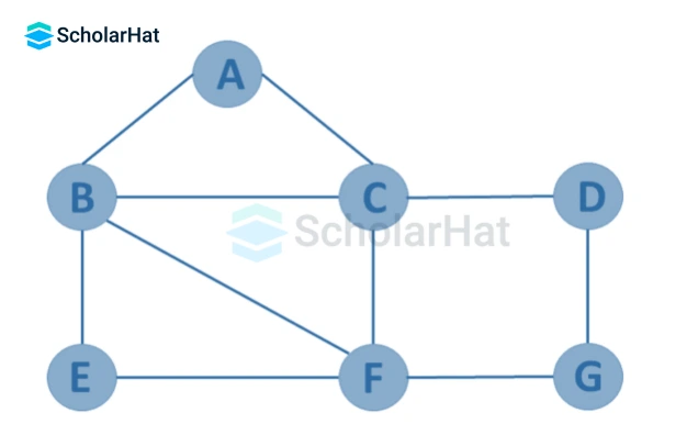
1. Finite Graph

If the graph, G=(V, E) has a finite number of edges and vertices, it is a finite graph. In other words, both the number of vertices and the number of edges in a finite graph are limited and can be counted.

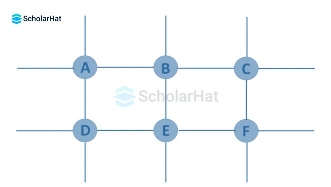
2. Infinite Graph

If the graph G=(V, E) has an infinite number of edges and vertices, it is an infinite graph.

3. Trivial Graph

If a finite graph G=(V, E) has just one vertex and no edges, it is referred to as trivial. It is also known as a singleton graph or a single vertex graph.

4. Simple Graph

A graph G=(V, E) is a simple one if each pair of nodes or vertices contains just one edge. In order to represent one-to-one interactions between two elements, there is only one edge connecting two vertices.

5. Multi Graph

A graph G=(V, E) is referred to as a multigraph if it has some parallel edges between two vertices but doesn't contain any self-loop. An edge of a graph that starts from a vertex and ends at the same vertex is called a loop or a self-loop.

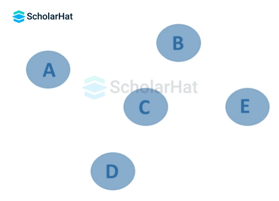
6. Null Graph

It's a revised version of a trivial graph. A graph G=(V, E) is a null graph if it has many vertices but none of them are connected by any edges. A null graph can also be referred to as an edgeless graph, an isolated graph, or a discrete graph.

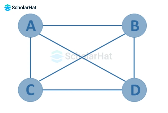
7. Complete Graph

A simple graph G=(V, E) with n vertices is also called a complete graph if the degree of each vertex is n-1, i.e. one vertex is attached with n-1 edges or the rest of the vertices in the graph. A complete graph is also called a Full Graph.

8. Pseudo Graph

A pseudograph exists when a graph G= (V, E) contains some self-loop in addition to some multiple edges.

9. Regular Graph

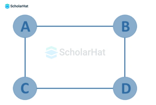
10. Weighted Graph

A graph G=(V, E) in which edges have weights or costs associated with them is a weighted graph.

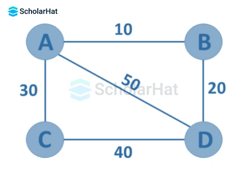
Graph Representation Using Adjacency List

• Add Vertex
• Add Edge
• Display the Graph

Example

class Graph:
    def __init__(self):
        self.graph = {}
        
    def add_vertex(self, vertex):
        if vertex not in self.graph:
            self.graph[vertex] = []
        else:
            print(f"Vertex {vertex} already exists.")
            
    def add_edge(self, vertex1, vertex2):
        if vertex1 in self.graph and vertex2 in self.graph:
            self.graph[vertex1].append(vertex2)
            self.graph[vertex2].append(vertex1)
        else:
            print("One or both vertices not found.")
    
    def display(self):
        for vertex in self.graph:
            print(vertex, ":", self.graph[vertex])

# Example usage
if __name__ == "__main__":
    g = Graph()
    
    # Adding vertices
    g.add_vertex("A")
    g.add_vertex("B")
    g.add_vertex("C")
    g.add_vertex("D")
    
    # Adding edges
    g.add_edge("A", "B")
    g.add_edge("A", "C")
    g.add_edge("B", "D")
    g.add_edge("C", "D")
    
    # Display the graph
    g.display()

Output

A : ['B', 'C']
B : ['A', 'D']
C : ['A', 'D']
D : ['B', 'C']

Explanation

Here, The Graph class contains methods to add vertices, add edges, and display the graph. after that,Adds a vertex to the graph. If the vertex already exists, it notifies the user. Then addan edge between two vertices. and finally,it Prints the adjacency list representation of the graph.

Properties of Non-Linear Data Structures

• When the data elements are not present in the contiguous memory locations, the non-linear data structure is utilized to store the combined data pieces.
• It is a productive method for arranging and storing the data.
• By giving each data element enough memory, the nonlinear minimizes memory space wastage.
• In contrast, when we define the size of an array, memory space is allotted to it, if we decide not to keep the elements until the array's range, the memory that remains is squandered.
• In order to get around this, we will move between nodes using a non-linear data structure.

Conclusion

In this tutorial, we saw the non-linear Data Structures including Trees and graphs in-depth, and also the Properties of Non-Linear Data Structures. To test your practical understanding of these two techniques, enroll in our Best Data Structures And Algorithms Course.