27
MarSpanning Tree and Minimum Spanning Tree in Data Structures - Kruskal's and Prim's Algorithms
Spanning Tree in Data Structures: An Overview
We have learned about graphs in the Graphs in Data Structures tutorial. In this DSA tutorial, we will learn about a subgraph, that contains all the vertices of a graph. It is known as a spanning tree. We will understand minimum spanning trees, Prim's Algorithm, Kruskal’s Algorithm, etc.
Build a strong foundation for high-paying tech roles with DSA expertise. Enroll in our Free DSA Course today!
What is a Spanning Tree in Data Structures?
It is a sub-graph of an undirected connected graph, which includes all the vertices of the graph with a minimal set of edges. It may or may not be weighted. Therefore a spanning tree does not have cycles and a graph may have multiple spanning trees. It cannot be disconnected.
Characteristics of a Spanning Tree
- Connectivity: A spanning tree must connect all the vertices of the original graph. This means that there is a path between any two vertices in the spanning tree.
- Acyclicity: A spanning tree is an acyclic graph, which means it contains no cycles. There are no closed loops or circuits in a spanning tree. It is a maximally acyclic sub-graph, which means if we add an edge to the spanning tree then it becomes cyclic.
- Minimal connected subgraph: A spanning tree is the smallest connected subgraph that can be formed from the original graph while including all of its vertices. Removing any edge from the spanning tree would disconnect the graph.
- Edges and Vertices: All possible spanning trees for graph G have the same number of edges and vertices.
- Spanning tree weight: If the original graph is weighted, where each edge has a numerical weight, the weight of a spanning tree is defined as the sum of the weights of all its edges. There may be multiple spanning trees for a given graph, and their weights can vary.
Mathematical Properties of a Spanning Tree
- The number of edges in a spanning tree is equal to the number of nodes or vertices minus one i.e. n-1
- A spanning tree can be constructed from a complete graph by removing a maximum of e - n + 1 edges.
- The total number of spanning trees with n vertices that can be created from a complete graph is equal to n^(n-2).
Example of a Spanning Tree
Let's suppose the original graph is:
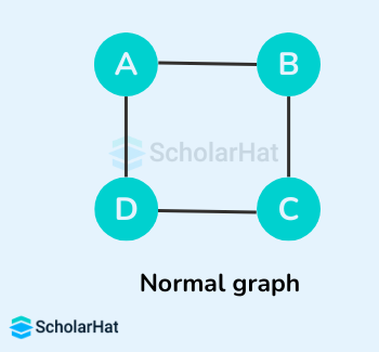
Some of the possible spanning trees that can be created from the above graph are:
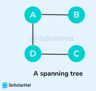
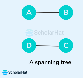
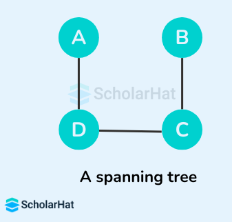
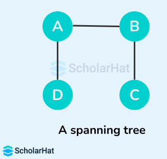
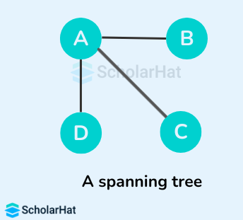
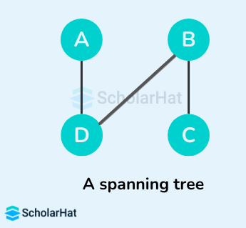
Read More - Data Structure Interview Questions for Freshers
Applications of Spanning Trees
- Network Design: In network engineering, spanning trees are used to construct efficient and fault-tolerant network topologies. Spanning tree algorithms, such as the Spanning Tree Protocol (STP) and its variants, help to eliminate loops in Ethernet networks and ensure that there is a single path between any two nodes in the network.
- Broadcast Storm Prevention: Spanning tree algorithms help prevent broadcast storms by identifying and blocking redundant paths in the network, thereby creating a loop-free topology.
- Routing: Spanning trees can be used as a basis for routing algorithms. By constructing a minimum spanning tree (MST) of a network, it is possible to determine the most efficient path between any two nodes.
- Network Monitoring: Spanning trees can be employed for network monitoring and analysis. By capturing the network traffic on each link of the spanning tree, it becomes easier to monitor the performance, identify bottlenecks, and analyze network behavior.
- Redundancy and High Availability: Spanning trees allow for the creation of redundant links in a network. By utilizing redundant links, network administrators can ensure high availability and fault tolerance. In the event of a link or switch failure, the spanning tree algorithm dynamically reroutes traffic through alternative paths, minimizing downtime and maintaining connectivity.
- Sensor Networks: Spanning trees find applications in wireless sensor networks (WSNs), where sensors are deployed to gather data in various environments.
- Clustering and Hierarchical Structures: Spanning trees can be utilized in data analysis and clustering algorithms. By constructing a minimum spanning tree of a dataset, it is possible to identify hierarchical structures and clustering patterns within the data, providing insights into the relationships between data points.
Minimum Spanning Tree
A minimum spanning tree(MST) is a subset of the edges of a connected, weighted graph that connects all the vertices with the minimum total edge weight. In other words, it is a tree that spans all the vertices of the graph with the minimum possible sum of edge weights.
It is a spanning tree that has the minimum cost among all the possible spanning trees. The cost of the spanning tree is the sum of the weights of all the edges in the tree. For a given graph G a minimum spanning tree of a graph is unique if the weight of all the edges is distinct. Otherwise, there may be multiple possible minimum spanning trees.
Characteristics of a Minimum Spanning Tree
- A minimum spanning tree connects all the vertices in the graph, ensuring that there is a path between any pair of nodes.
- An MST is acyclic, i.e. it contains no cycles. This property ensures that it remains a tree and not a graph with loops.
- An MST with n vertices (where n is the number of vertices in the original graph) will have exactly n – 1 edges.
- An MST is optimal for minimizing the total edge weight, but it may not necessarily be unique.
- The cut property states that if you take any cut (a partition of the vertices into two sets) in the original graph and consider the minimum-weight edge that crosses the cut, that edge is part of the MST.
Example of a Minimum Spanning Tree
Let's suppose the initial graph is:
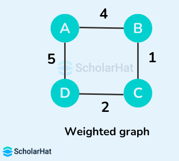
Some of the possible spanning trees from the above graph are:
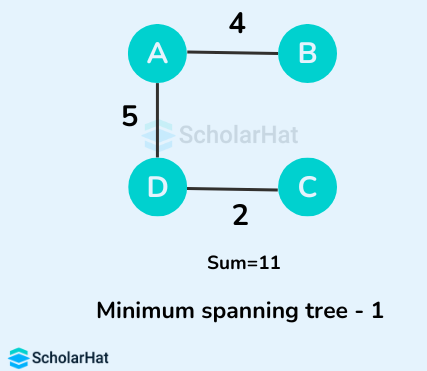
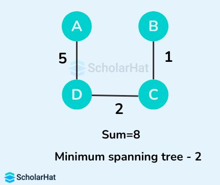
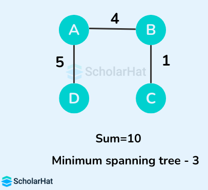
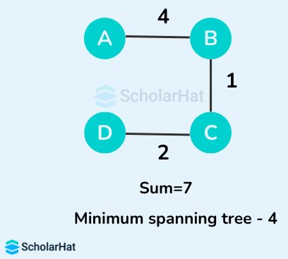
The minimum spanning tree from the above spanning trees is:
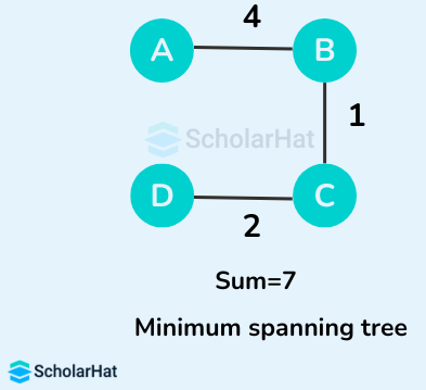
Applications of Minimum Spanning Trees
- A Minimum Spanning Tree is used for designing telecommunication networks and water supply networks.
- For designing Local Area Networks.
- To solve the Traveling salesman problem.
- Real-time face tracking and verification (i.e. locating human faces in a video stream).
- Minimum spanning trees can also be used to describe financial markets.
- Handwriting recognition of mathematical expressions.
- Curvilinear feature extraction in computer vision.
- For building or Connecting the roads among cities or villages at a minimal cost.
- Minimum Spanning Trees are used for clustering i.e. grouping of similar objects under one category and distinguishing from other categories.
Algorithms for Minimum Spanning Tree
The minimum spanning tree from a graph is found using the following algorithms:
- Kruskal's Algorithm
In Kruskal's algorithm, the spanning tree is constructed by adding the edges one by one. It falls under a class of algorithms called greedy algorithms that find the local optimum in the hopes of finding a global optimum. We start from the edges with the lowest weight and keep adding edges until we reach our goal.
Working of the Kruskal's Algorithm
- Sort all the edges of the graph in the increasing order of their weight.
- Pick the edge with the smallest weight.
- Check if it forms a cycle with the spanning tree formed so far.
- Include the current edge if it does not form any cycle.
- Otherwise, discard it.
- Repeat step 3 until there are n-1 edges in the spanning tree, where n is the total number of vertices in the graph.
Example of Kruskal's Algorithm
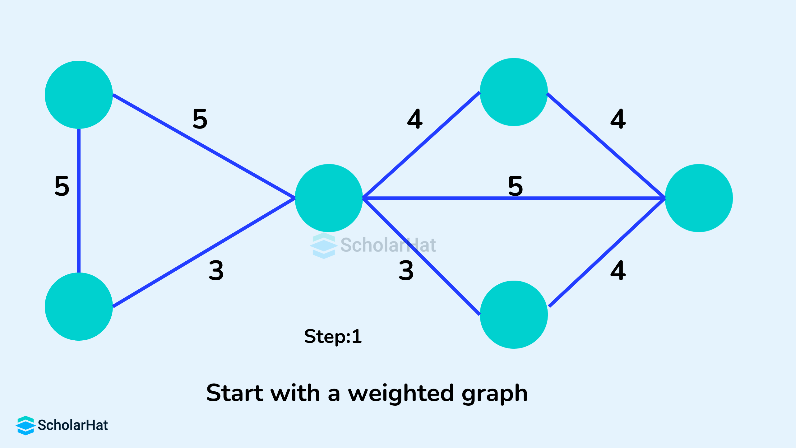
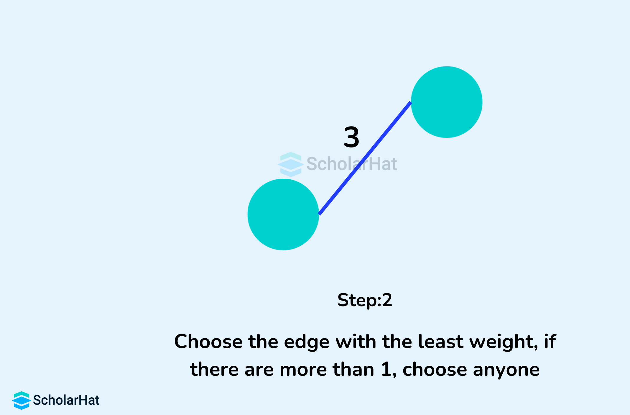
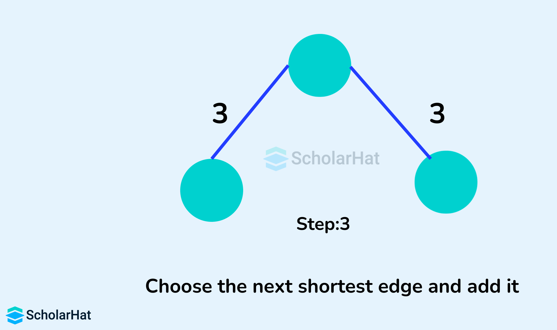
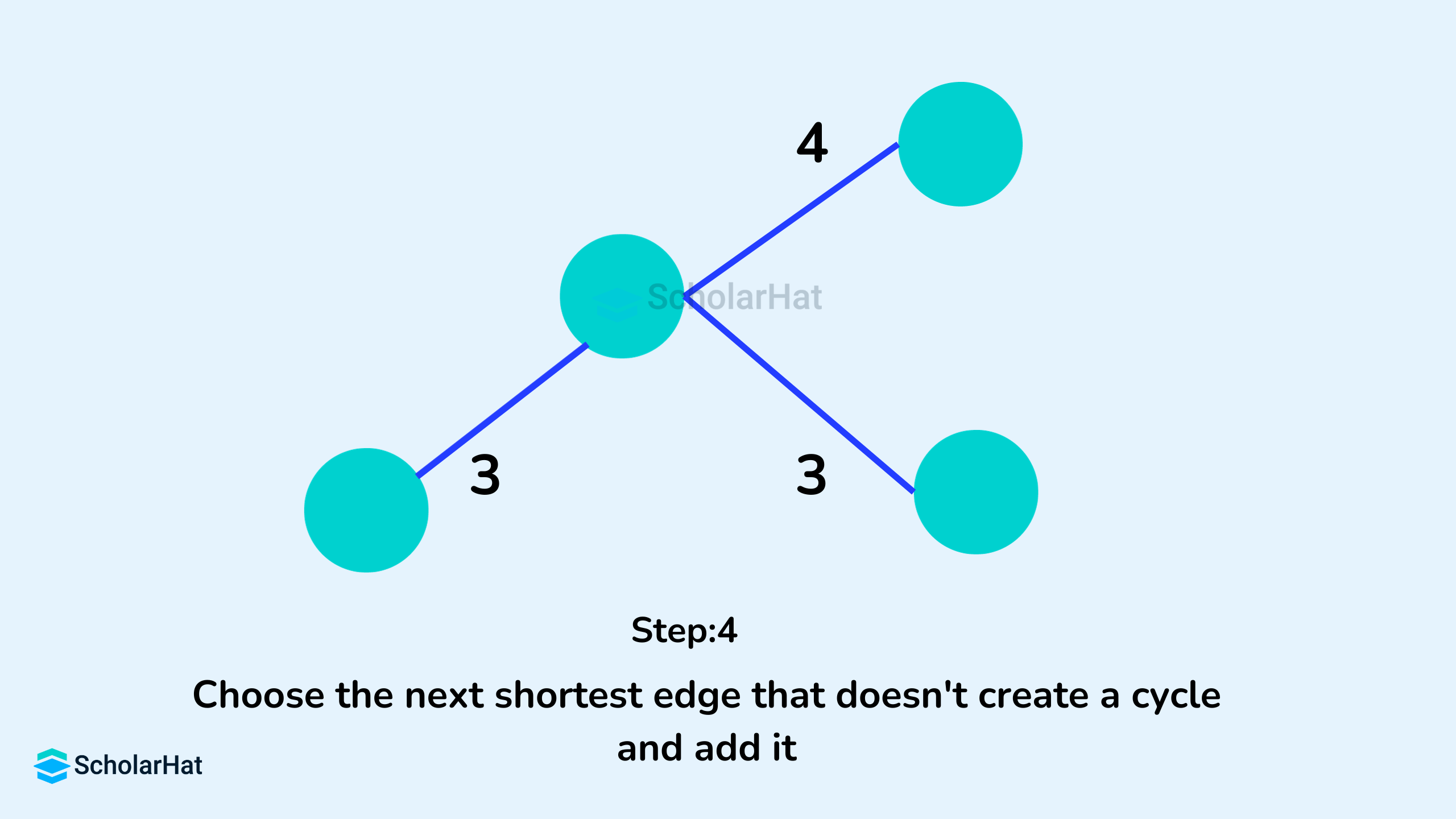
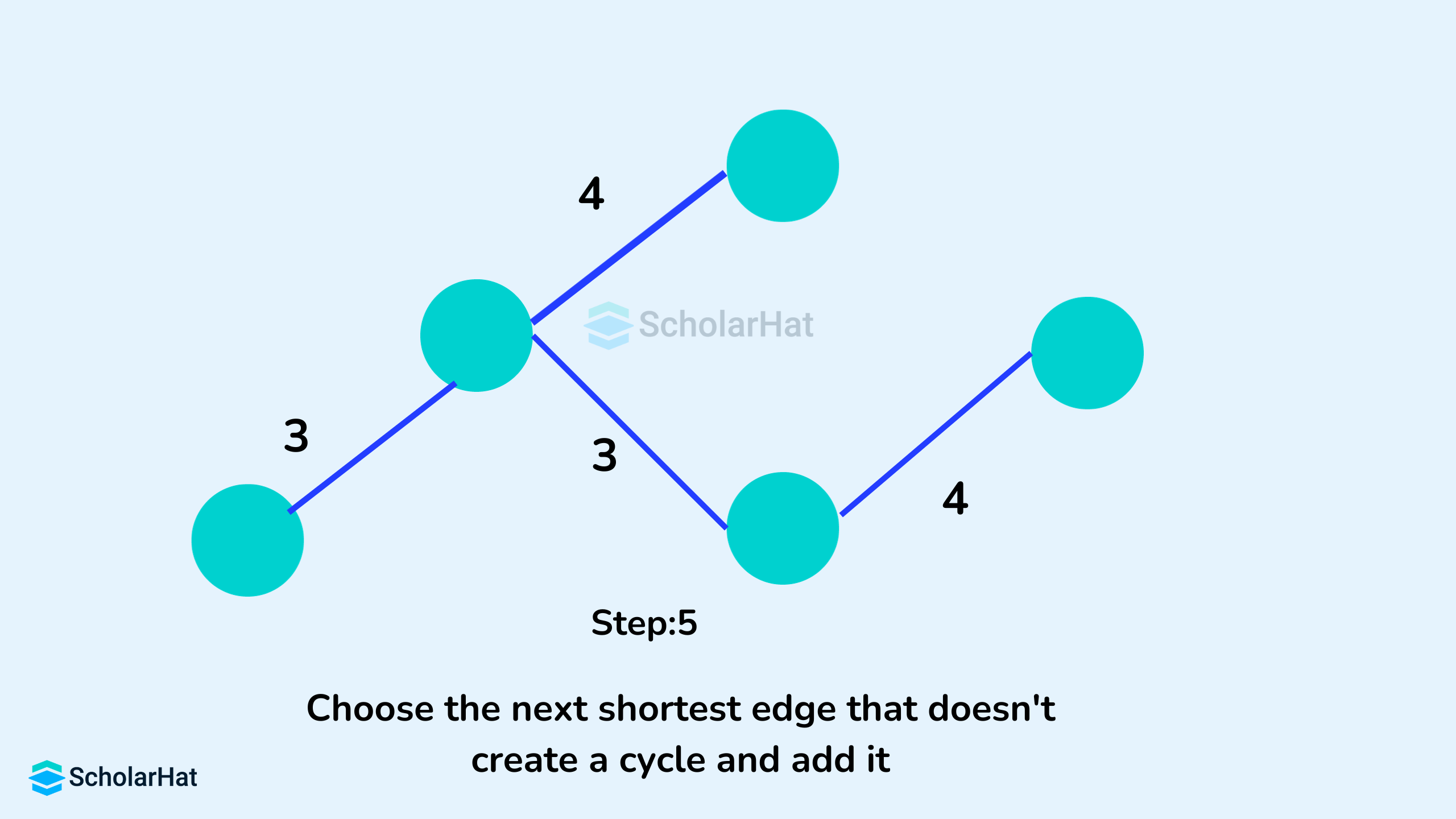

Kruskal's Algorithm Pseudocode
Any minimum spanning tree algorithm revolves around checking if adding an edge creates a loop or not. The most common way to find this out is an algorithm called Union FInd. The Union-Find algorithm divides the vertices into clusters and allows us to check if two vertices belong to the same cluster or not and hence decide whether adding an edge creates a cycle.
KRUSKAL(G):
A = ∅
For each vertex v ∈ G.V:
    MAKE-SET(v)
For each edge (u, v) ∈ G.E ordered by increasing order by weight(u, v):
    if FIND-SET(u) ≠ FIND-SET(v):
    A = A ∪ {(u, v)}
    UNION(u, v)
return A
Implementation of Kruskal's Algorithm in Different Programming Languages
class Graph:
    def __init__(self, vertices):
        self.V = vertices
        self.graph = []

    def add_edge(self, u, v, w):
        self.graph.append([u, v, w])

    # Search function
    def find(self, parent, i):
        if parent[i] == i:
            return i
        return self.find(parent, parent[i])

    def apply_union(self, parent, rank, x, y):
        xroot = self.find(parent, x)
        yroot = self.find(parent, y)
        if rank[xroot] < rank[yroot]:
            parent[xroot] = yroot
        elif rank[xroot] > rank[yroot]:
            parent[yroot] = xroot
        else:
            parent[yroot] = xroot
            rank[xroot] += 1

    #  Applying Kruskal algorithm
    def kruskal_algo(self):
        result = []
        i, e = 0, 0
        self.graph = sorted(self.graph, key=lambda item: item[2])
        parent = []
        rank = []
        for node in range(self.V):
            parent.append(node)
            rank.append(0)
        while e < self.V - 1:
            u, v, w = self.graph[i]
            i = i + 1
            x = self.find(parent, u)
            y = self.find(parent, v)
            if x != y:
                e = e + 1
                result.append([u, v, w])
                self.apply_union(parent, rank, x, y)
        print("Edge : Weight")
        for u, v, weight in result:
            print("%d - %d: %d" % (u, v, weight))


g = Graph(6)
g.add_edge(0, 1, 4)
g.add_edge(0, 2, 6)
g.add_edge(1, 2, 2)
g.add_edge(1, 0, 4)
g.add_edge(2, 0, 4)
g.add_edge(2, 1, 2)
g.add_edge(2, 3, 3)
g.add_edge(2, 5, 2)
g.add_edge(2, 4, 4)
g.add_edge(3, 2, 3)
g.add_edge(3, 4, 3)
g.add_edge(4, 2, 4)
g.add_edge(4, 3, 3)
g.add_edge(5, 2, 8)
g.add_edge(5, 4, 3)
g.kruskal_algo()
import java.util.*;

class Graph {
  class Edge implements Comparable {
    int src, dest, weight;

    public int compareTo(Edge compareEdge) {
      return this.weight - compareEdge.weight;
    }
  };

  // Union
  class subset {
    int parent, rank;
  };

  int vertices, edges;
  Edge edge[];

  // Graph creation
  Graph(int v, int e) {
    vertices = v;
    edges = e;
    edge = new Edge[edges];
    for (int i = 0; i < e; ++i)
      edge[i] = new Edge();
  }

  int find(subset subsets[], int i) {
    if (subsets[i].parent != i)
      subsets[i].parent = find(subsets, subsets[i].parent);
    return subsets[i].parent;
  }

  void Union(subset subsets[], int x, int y) {
    int xroot = find(subsets, x);
    int yroot = find(subsets, y);

    if (subsets[xroot].rank < subsets[yroot].rank)
      subsets[xroot].parent = yroot;
    else if (subsets[xroot].rank > subsets[yroot].rank)
      subsets[yroot].parent = xroot;
    else {
      subsets[yroot].parent = xroot;
      subsets[xroot].rank++;
    }
  }

  // Applying Krushkal Algorithm
  void KruskalAlgo() {
    Edge result[] = new Edge[vertices];
    int e = 0;
    int i = 0;
    for (i = 0; i < vertices; ++i)
      result[i] = new Edge();

    // Sorting the edges
    Arrays.sort(edge);
    subset subsets[] = new subset[vertices];
    for (i = 0; i < vertices; ++i)
      subsets[i] = new subset();

    for (int v = 0; v < vertices; ++v) {
      subsets[v].parent = v;
      subsets[v].rank = 0;
    }
    i = 0;
    while (e < vertices - 1) {
      Edge next_edge = new Edge();
      next_edge = edge[i++];
      int x = find(subsets, next_edge.src);
      int y = find(subsets, next_edge.dest);
      if (x != y) {
        result[e++] = next_edge;
        Union(subsets, x, y);
      }
    }
    System.out.println("Edge : Weight");
    for (i = 0; i < e; ++i)
      System.out.println(result[i].src + " - " + result[i].dest + ": " + result[i].weight);
  }

  public static void main(String[] args) {
    int vertices = 6; // Number of vertices
    int edges = 8; // Number of edges
    Graph G = new Graph(vertices, edges);

    G.edge[0].src = 0;
    G.edge[0].dest = 1;
    G.edge[0].weight = 4;

    G.edge[1].src = 0;
    G.edge[1].dest = 2;
    G.edge[1].weight = 4;

    G.edge[2].src = 1;
    G.edge[2].dest = 2;
    G.edge[2].weight = 2;

    G.edge[3].src = 2;
    G.edge[3].dest = 3;
    G.edge[3].weight = 3;

    G.edge[4].src = 2;
    G.edge[4].dest = 5;
    G.edge[4].weight = 2;

    G.edge[5].src = 2;
    G.edge[5].dest = 4;
    G.edge[5].weight = 4;

    G.edge[6].src = 3;
    G.edge[6].dest = 4;
    G.edge[6].weight = 3;

    G.edge[7].src = 5;
    G.edge[7].dest = 4;
    G.edge[7].weight = 3;
    G.KruskalAlgo();
  }
}
#include <algorithm>
#include <iostream>
#include <vector>
using namespace std;

#define edge pair

class Graph {
   private:
  vector > G;  // graph
  vector > T;  // mst
  int *parent;
  int V;  // number of vertices/nodes in graph
   public:
  Graph(int V);
  void AddWeightedEdge(int u, int v, int w);
  int find_set(int i);
  void union_set(int u, int v);
  void kruskal();
  void print();
};
Graph::Graph(int V) {
  parent = new int[V];

  //i 0 1 2 3 4 5
  //parent[i] 0 1 2 3 4 5
  for (int i = 0; i < V; i++)
    parent[i] = i;

  G.clear();
  T.clear();
}
void Graph::AddWeightedEdge(int u, int v, int w) {
  G.push_back(make_pair(w, edge(u, v)));
}
int Graph::find_set(int i) {
  // If i is the parent of itself
  if (i == parent[i])
    return i;
  else
    // Else if i is not the parent of itself
    // Then i is not the representative of his set,
    // so we recursively call Find on its parent
    return find_set(parent[i]);
}

void Graph::union_set(int u, int v) {
  parent[u] = parent[v];
}
void Graph::kruskal() {
  int i, uRep, vRep;
  sort(G.begin(), G.end());  // increasing weight
  for (i = 0; i < G.size(); i++) {
    uRep = find_set(G[i].second.first);
    vRep = find_set(G[i].second.second);
    if (uRep != vRep) {
      T.push_back(G[i]);  // add to tree
      union_set(uRep, vRep);
    }
  }
}
void Graph::print() {
  cout << "Edge :" << " Weight" << endl;
  for (int i = 0; i < T.size(); i++) {
    cout << T[i].second.first << " - " << T[i].second.second << " : "
       << T[i].first;
    cout << endl;
  }
}
int main() {
  Graph g(6);
  g.AddWeightedEdge(0, 1, 4);
  g.AddWeightedEdge(0, 2, 6);
  g.AddWeightedEdge(1, 2, 2);
  g.AddWeightedEdge(1, 0, 4);
  g.AddWeightedEdge(2, 0, 4);
  g.AddWeightedEdge(2, 1, 2);
  g.AddWeightedEdge(2, 3, 3);
  g.AddWeightedEdge(2, 5, 2);
  g.AddWeightedEdge(2, 4, 4);
  g.AddWeightedEdge(3, 2, 3);
  g.AddWeightedEdge(3, 4, 3);
  g.AddWeightedEdge(4, 2, 4);
  g.AddWeightedEdge(4, 3, 3);
  g.AddWeightedEdge(5, 2, 8);
  g.AddWeightedEdge(5, 4, 3);
  g.kruskal();
  g.print();
  return 0;
}
Output
Edge : Weight
1 - 2: 2
2 - 5: 2
2 - 3: 3
3 - 4: 3
0 - 1: 4
Applications of Kruskal's Algorithm
- To lay electrical wiring
- In computer network (LAN connection)
- Prim's Algorithm
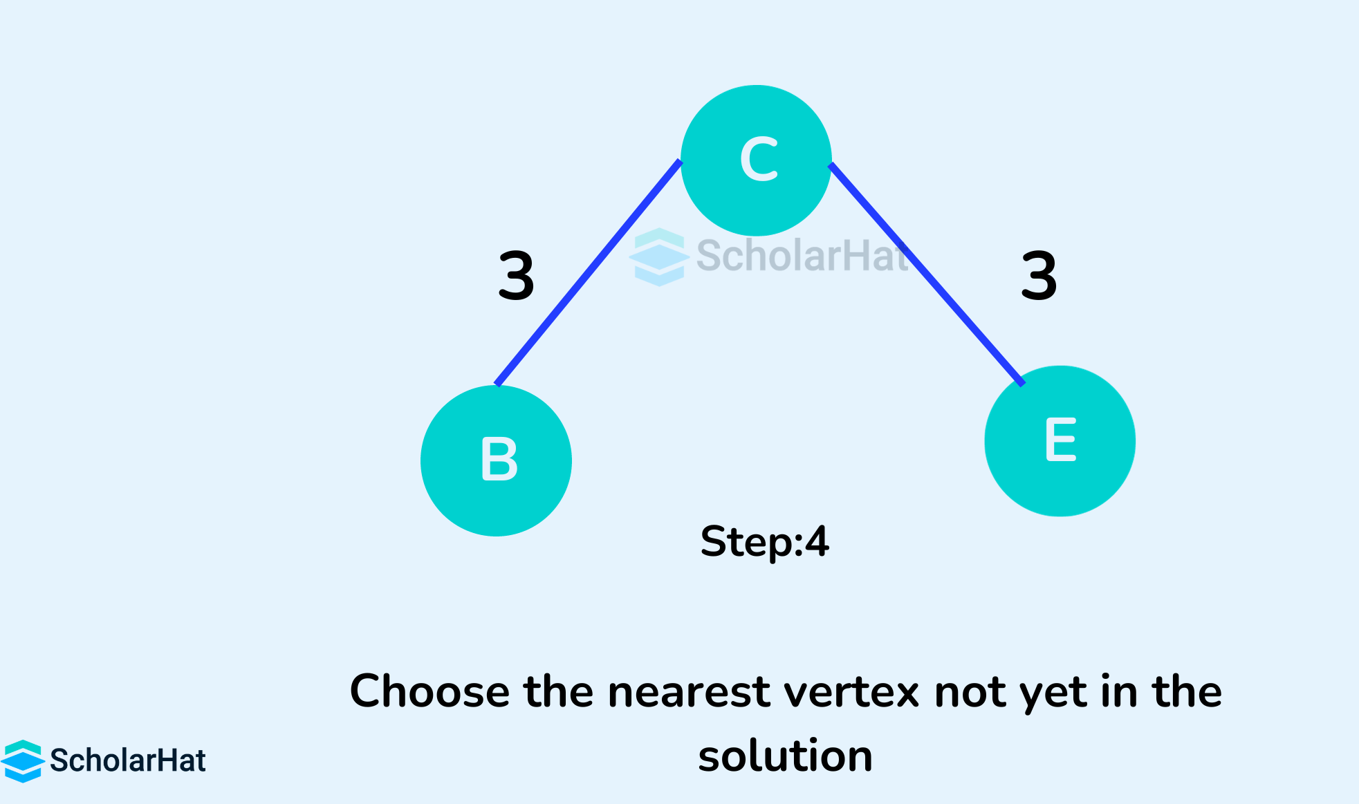
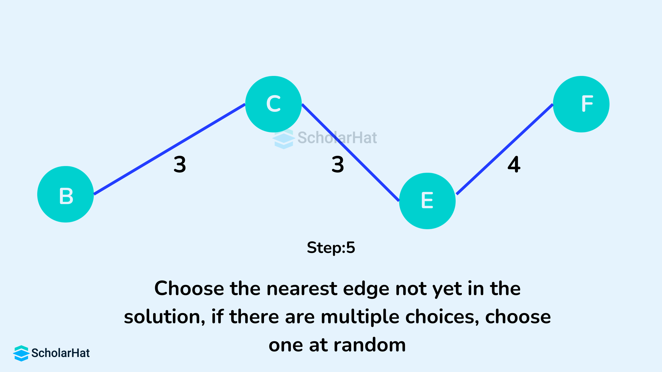
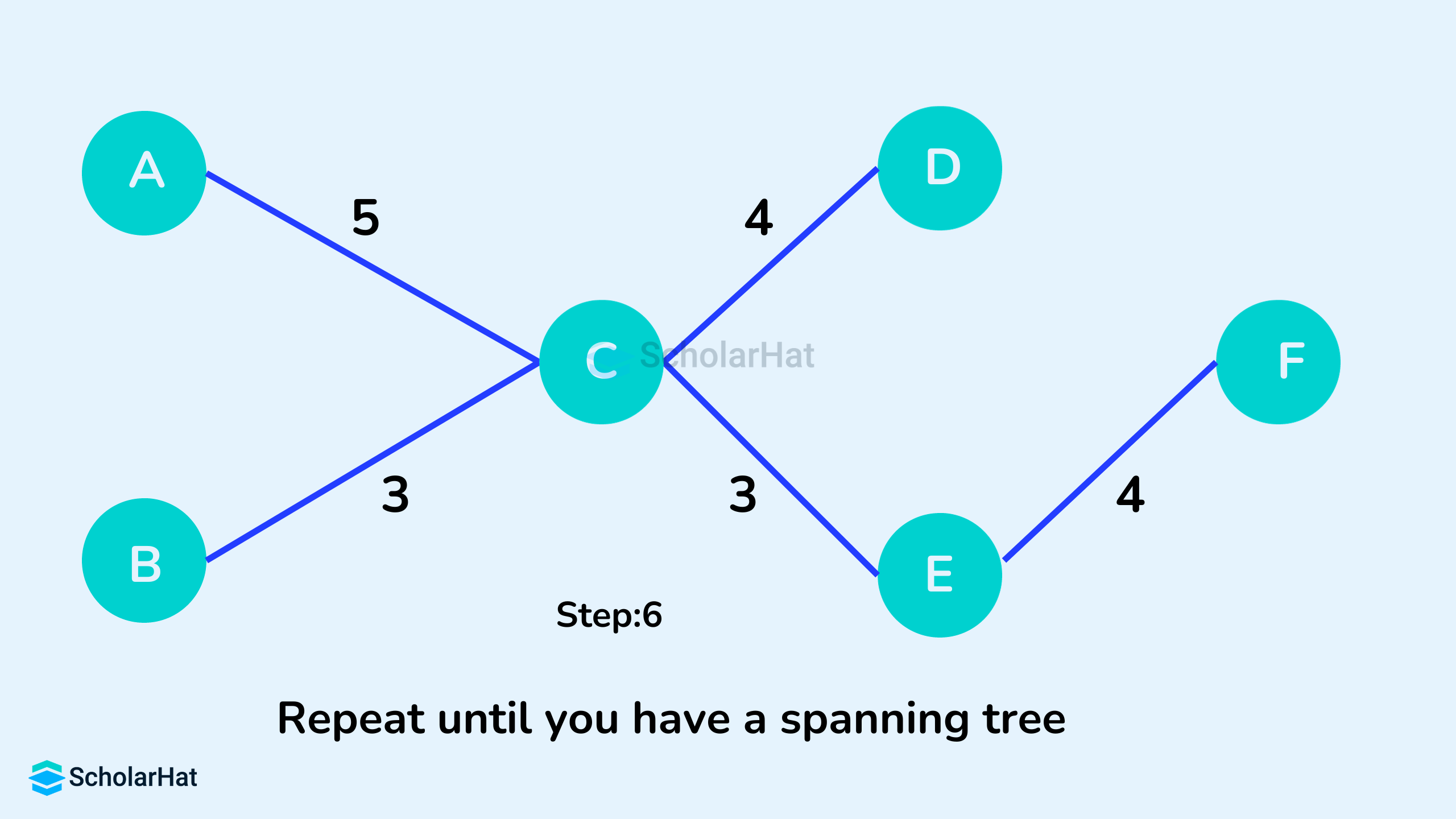
It takes a graph as input and finds the subset of the edges of that graph which form a tree that includes every vertex and has the minimum sum of weights among all the trees that can be formed from the graph. It falls under a class of algorithms called greedy algorithms that find the local optimum in the hopes of finding a global optimum. We start from one vertex and keep adding edges with the lowest weight until we reach our goal.
Unlike Kruskal's algorithm, Prim's algorithm treats the nodes as a single tree and keeps on adding new nodes to the spanning tree from the given graph.
Working of the Prim's Algorithm
- Initialize the minimum spanning tree with a vertex chosen at random.
- Find all the edges that connect the tree to new vertices, find the minimum, and add it to the tree.
- Keep repeating step 2 until we get a minimum spanning tree
Example of Prim's Algorithm
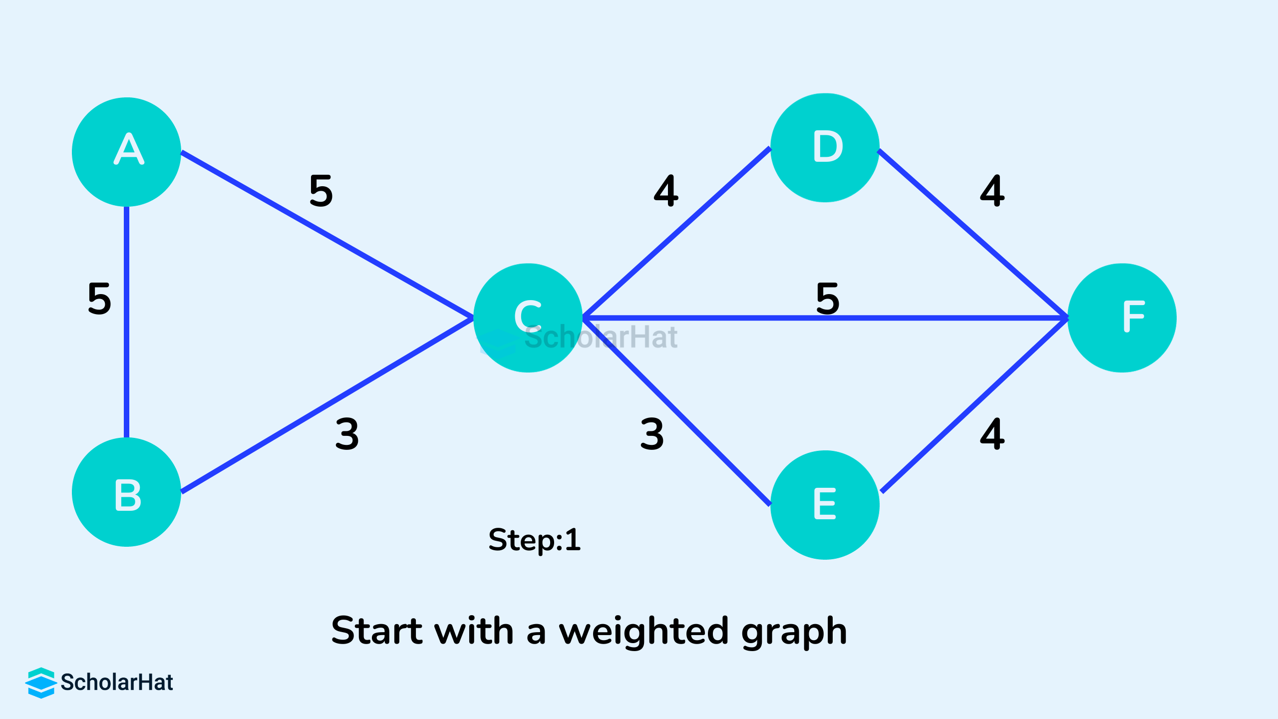

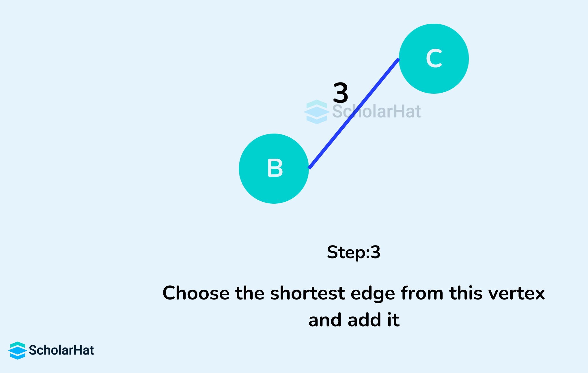
Prim's Algorithm Pseudocode
It illustrates how we create two sets of vertices U and V-U. U contains the list of vertices that have been visited and V-U contains the list of vertices that haven't. One by one, we move vertices from set V-U to set U by connecting the least-weight edge. To efficiently select the minimum weight edge for each iteration, this algorithm uses a priority queue to store the vertices sorted by their minimum edge weight currently.
T = ∅;
U = { 1 };
while (U ≠ V)
    let (u, v) be the lowest cost edge such that u ∈ U and v ∈ V - U;
    T = T ∪ {(u, v)}
    U = U ∪ {v}
Implementation of Prim's Algorithm in Different Programming Languages
INF = 9999999
# number of vertices in graph
V = 5
# create a 2d array of size 5x5
# for adjacency matrix to represent graph
G = [[0, 9, 75, 0, 0],
     [9, 0, 95, 19, 42],
     [75, 95, 0, 51, 66],
     [0, 19, 51, 0, 31],
     [0, 42, 66, 31, 0]]
# create a array to track selected vertex
# selected will become true otherwise false
selected = [0, 0, 0, 0, 0]
# set number of edge to 0
no_edge = 0
# the number of egde in minimum spanning tree will be
# always less than(V - 1), where V is number of vertices in
# graph
# choose 0th vertex and make it true
selected[0] = True
# print for edge and weight
print("Edge : Weight")
while (no_edge < V - 1):
    # For every vertex in the set S, find the all adjacent vertices
    #, calculate the distance from the vertex selected at step 1.
    # if the vertex is already in the set S, discard it otherwise
    # choose another vertex nearest to selected vertex  at step 1.
    minimum = INF
    x = 0
    y = 0
    for i in range(V):
        if selected[i]:
            for j in range(V):
                if ((not selected[j]) and G[i][j]):
                    # not in selected and there is an edge
                    if minimum > G[i][j]:
                        minimum = G[i][j]
                        x = i
                        y = j
    print(str(x) + "-" + str(y) + " : " + str(G[x][y]))
    selected[y] = True
    no_edge += 1
import java.util.Arrays;

class PGraph {

  public void Prim(int G[][], int V) {

    int INF = 9999999;

    int no_edge; // number of edge

    // create a array to track selected vertex
    // selected will become true otherwise false
    boolean[] selected = new boolean[V];

    // set selected false initially
    Arrays.fill(selected, false);

    // set number of edge to 0
    no_edge = 0;

    // the number of egde in minimum spanning tree will be
    // always less than (V -1), where V is number of vertices in
    // graph

    // choose 0th vertex and make it true
    selected[0] = true;

    // print for edge and weight
    System.out.println("Edge : Weight");

    while (no_edge < V - 1) {
      // For every vertex in the set S, find the all adjacent vertices
      // , calculate the distance from the vertex selected at step 1.
      // if the vertex is already in the set S, discard it otherwise
      // choose another vertex nearest to selected vertex at step 1.

      int min = INF;
      int x = 0; // row number
      int y = 0; // col number

      for (int i = 0; i < V; i++) {
        if (selected[i] == true) {
          for (int j = 0; j < V; j++) {
            // not in selected and there is an edge
            if (!selected[j] && G[i][j] != 0) {
              if (min > G[i][j]) {
                min = G[i][j];
                x = i;
                y = j;
              }
            }
          }
        }
      }
      System.out.println(x + " - " + y + " :  " + G[x][y]);
      selected[y] = true;
      no_edge++;
    }
  }

  public static void main(String[] args) {
    PGraph g = new PGraph();

    // number of vertices in grapj
    int V = 5;

    // create a 2d array of size 5x5
    // for adjacency matrix to represent graph
    int[][] G = { { 0, 9, 75, 0, 0 }, { 9, 0, 95, 19, 42 }, { 75, 95, 0, 51, 66 }, { 0, 19, 51, 0, 31 },
        { 0, 42, 66, 31, 0 } };

    g.Prim(G, V);
  }
}
#include
#include
using namespace std;

#define INF 9999999

// number of vertices in grapj
#define V 5

// create a 2d array of size 5x5
//for adjacency matrix to represent graph

int G[V][V] = {
  {0, 9, 75, 0, 0},
  {9, 0, 95, 19, 42},
  {75, 95, 0, 51, 66},
  {0, 19, 51, 0, 31},
  {0, 42, 66, 31, 0}};

int main() {
  int no_edge;  // number of edge

  // create a array to track selected vertex
  // selected will become true otherwise false
  int selected[V];

  // set selected false initially
  memset(selected, false, sizeof(selected));

  // set number of edge to 0
  no_edge = 0;

  // the number of egde in minimum spanning tree will be
  // always less than (V -1), where V is number of vertices in
  //graph

  // choose 0th vertex and make it true
  selected[0] = true;

  int x;  //  row number
  int y;  //  col number

  // print for edge and weight
  cout << "Edge"
     << " : "
     << "Weight";
  cout << endl;
  while (no_edge < V - 1) {
    //For every vertex in the set S, find the all adjacent vertices
    // , calculate the distance from the vertex selected at step 1.
    // if the vertex is already in the set S, discard it otherwise
    //choose another vertex nearest to selected vertex  at step 1.

    int min = INF;
    x = 0;
    y = 0;

    for (int i = 0; i < V; i++) {
      if (selected[i]) {
        for (int j = 0; j < V; j++) {
          if (!selected[j] && G[i][j]) {  // not in selected and there is an edge
            if (min > G[i][j]) {
              min = G[i][j];
              x = i;
              y = j;
            }
          }
        }
      }
    }
    cout << x << " - " << y << " :  " << G[x][y];
    cout << endl;
    selected[y] = true;
    no_edge++;
  }

  return 0;
}
Output
Edge : Weight
0-1 : 9
1-3 : 19
3-4 : 31
3-2 : 51
Applications of Prim's Algorithm
- Laying cables of electrical wiring
- In network designed
- To make protocols in network cycles
Complexity Analysis of Kruskal's and Prim's Algorithms
- For the Adjacency List representation of the graph
Time Complexity Space Complexity Prim's Algorithm O((V + E)logV) O(V + E) Kruskal's Algorithm O(ElogE + ELogV) O(V + E) - For the Adjacency Matrix representation of the graph,
Time Complexity Space Complexity Prim's Algorithm O(V^2) O(V^2) Kruskal's Algorithm O(V^2) O(V^2)
Here, E is the number of edges and V is the number of vertices in graph G.
Difference between Kruskal's and Prim's Algorithms
| Prim’s Algorithm | Kruskal’s Algorithm |
| It starts to build the Minimum Spanning Tree from any vertex in the graph. | It starts to build the Minimum Spanning Tree from the vertex carrying the minimum weight in the graph. |
| It traverses one node more than one time to get the minimum distance. | It traverses one node only once. |
| It has a time complexity of O(V^2), V being the number of vertices, and can be improved up to O(E log V) using Fibonacci heaps. | It has a time complexity is O(E log V), V being the number of vertices. |
| Prim’s algorithm gives connected components as well and it works only on connected graphs. | Kruskal’s algorithm can generate a forest(disconnected components) at any instant as well as it can work on disconnected components |
| Prim’s algorithm runs faster in dense graphs. | Kruskal’s algorithm runs faster in sparse graphs. |
| Applications are Travelling Salesman Problem, Network for roads and Rail tracks connecting all the cities, etc. | Applications are LAN connection, TV Network, etc. |
| Prim’s algorithm prefers list data structures. | Kruskal’s algorithm prefers heap data structures. |
Summary
A spanning tree is an essential data structure that offers the advantage of locating connections quickly and within a limited search space. It allows for efficient intra-connectivity while maintaining the minimalist tree structure, making it useful for environments where merging data points is a common activity. You need to practice the learned concepts to fully understand this topic.
Only 2% of Java Developers become Solution Architects. Don’t get left behind—Enroll now in our Java Architect Certification and secure your career growth & 60% higher salary potential.
FAQs
- Laying cables of electrical wiring
- In network designed
- To make protocols in network cycles
Take our Datastructures skill challenge to evaluate yourself!

In less than 5 minutes, with our skill challenge, you can identify your knowledge gaps and strengths in a given skill.


